How to Rank in Excel

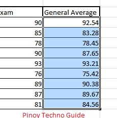
Teachers use Microsoft excel in computing the grades of their students. This makes it more convenient to the teacher than manually compute grades.

However, there are some tasks that teachers find difficult to make in MS Excel. One of these is RANKING. After getting the General Average of the students, many teachers will manually look for the highest General Average to mark that student for the First Honors. It might not be that hard if you will do it only once, but doing it everytime the honors will be selected just doesn’t feel right. You have MS Excel, why can’t it rank these students for you?

Here are some simple baby steps to RANK your students automatically in MS Excel:

1. If you already have the General Average of your students, select all of it. Select all the Averages of all your students.
2. We have to name these values so that we can use them as a single item, a single entity. Go to Formulas > Define Name. You should see a dialogue box pop up.
3. On the Name box, write any name you want. general_average will be okay. Then click OK.
4. Now make a new column and name it Rank.
5. On the cell below the heading Rank, input this formula: =RANK(F4,general_average,0)

      6.  Let’s look at that formula one by one. =RANK(F4,general_average,0)

Of course the formula must begin with “=”. Don’t ever forget that. RANK means that you will rank the given values. F4 is the name of the cell where the general average of the student is found. general_average is the name of all the general averages of your students. 0 is the order of the ranking which means descending. The one with the highest general average will be ranked as number one.
Copy the formula in the entire Rank column and you will get the ranks of all the students.
That’s it!